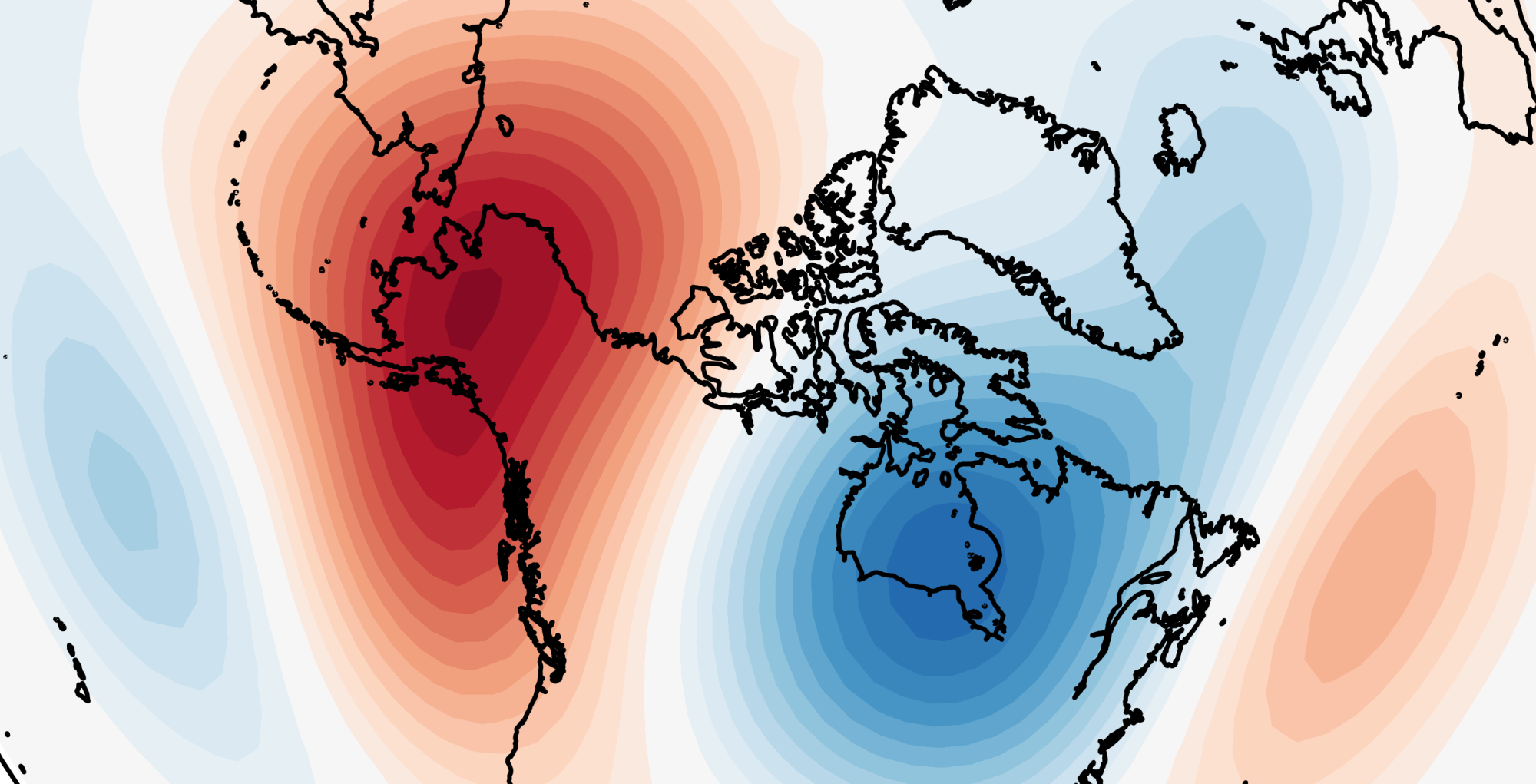
I’ve recently added some additional products from the NCEP Climate Forecast System version 2 (CFSv2) to my site — namely, forecasts of the weekly-average 500 hPa geopotential height anomalies for the next 4 weeks, and forecasts of the monthly-mean 700 hPa geopotential height anomalies over the next 6 months. These sit alongside the 44 day ensemble-plume forecasts of 10 hPa 60°N zonal-mean zonal wind (which are a bit less interesting in the summer, to say the least!). Though the new products are just re-plotted versions of those available here, I hope they’re a bit cleaner and easier to interpret.

Now, every time I mention CFSv2 forecasts, someone invariably replies with “but it’s garbage beyond week 3” or “the model changes day-to-day, just guesswork”. If this is true, why have I bothered putting effort into making CFSv2 charts? The answer is that CFSv2 isn’t actually as bad as some people find it to be. Part of my PhD involves looking at the longer-range forecasts from multiple modelling centres around the world – including CFSv2 – and in what I’ve seen (some of which is in a few upcoming papers), CFSv2 doesn’t stick out as being rubbish. Far from it, in fact. That doesn’t mean it’s the best — it isn’t — but it’s worthwhile to look at (especially as we all have access to it), and it does quite well considering it is 9 years old.
As it’s a NOAA forecast model, CFSv2 data is freely available – unlike that of ECMWF or the UK Met Office. I would argue this is a key reason behind why some find CFSv2 to be so poor; that reason being that it is relatively easy to go and see individual runs of the model, even individual ensemble members, and watch them change massively day to day.
All that does is prove, in a qualitative sense, that the atmosphere is not deterministically predictable beyond about a fortnight. We’ve known this for some time.
Predicting the atmosphere at longer lead-times is thus inherently probabilistic. CFSv2 produces probabilistic forecasts by running “lagged” ensembles — that is, accumulating ensemble runs over some period of time to generate a larger ensemble that has sampled different uncertainties in its starting conditions. The Met Office also use this approach. ECMWF use “burst” ensembles, where the entire (large) ensemble starts at the same time (with the hope that the larger ensemble samples the uncertainty by being large). There’s not necessarily a right way to do it, but experience seems to suggest lagged ensembles “jump” less. I don’t have anything to rigorously defend that with.
Anyway, I digress. Various examples of the lagged ensemble approach are used in my CFSv2 charts. The U10-60 forecast uses a 16-member ensemble constructed by taking the 4-member ensembles produced 4 times a day (00, 06, 12, 18Z). The weekly 500 hPa anomalies use the same approach. Meanwhile, the seasonal 700 hPa anomalies use 10 days of runs. The forecasts from CFSv2 which contribute to the C3S seasonal database use an entire month of runs!
Hidden within all this, is the random noise that (thanks to NCEP’s freely available data policy) people are able to go and see on the Internet, and thus conclude that CFSv2 is shit. Meanwhile, the Met Office’s GloSea5 is also jumping around, but that’s hidden from public view (though, yes, GloSea5 is indeed better than CFSv2). Even when lagged ensembles are considered, a 16-member ensemble that is run daily will still shift around a fair bit, so a user should look for patterns between the different runs.
Sometimes, the criticism that CFSv2 almost exclusively receives is in truth a more general criticism of longer-term forecast skill being poor.
Additionally, models have mean-state biases. In the best models, this is small, but it’s always there. What this means is that, over the period of a forecast, a model will “drift” toward its own climatology. For example, in CFSv2, in the stratosphere, the model drifts toward having a weak polar vortex. This doesn’t mean it is actually predicting a weak polar vortex. Extended-range forecasts have to address this. However, biases can dynamically interfere with what the model can then predict (e.g. if the model has stratospheric easterlies, how would it then forecast an SSW correctly?), so large biases are inherently bad no matter what is done to account for them.

One way to account for biases is to express anomalies with respect to the model’s climatology (hence why these CFSv2 charts say “1999-2010 model climatology”), which is produced by re-running the model in the past (hindcasts) and creating a climatology which depends on the initialisation date and the lead-time. Or, we can express the actual magnitudes (e.g. 10 hPa zonal winds), but subtract the bias (by computing the difference between the model’s climatology and a reanalysis like ERA5). My CFSv2 stratosphere charts do the latter (during November-March as this is when the vortex is active), and this can make a significant difference to the predictions.
It is absolutely not appropriate to put a raw model forecast alongside a reanalysis climatology and compare the two, unless you know what the model bias is.
I hope this was informative and helps explain why looking at CFSv2 isn’t a waste of time — so long as you do it properly 😉
Thanks for posting tthis