The many faces of the NAO

To describe the large-scale atmospheric circulation on a given day, we often use patterns. An example pattern is the North Atlantic Oscillation (NAO), which I’m going to focus on here. In general, the NAO is a measure of the pressure difference between the Azores high and Iceland low, and is thus intrinsically related to the strength and position of the North Atlantic eddy driven jet. Now, there are several different methods which can be used to define the NAO, which can be potentially confusing. I’ll describe some of these here.

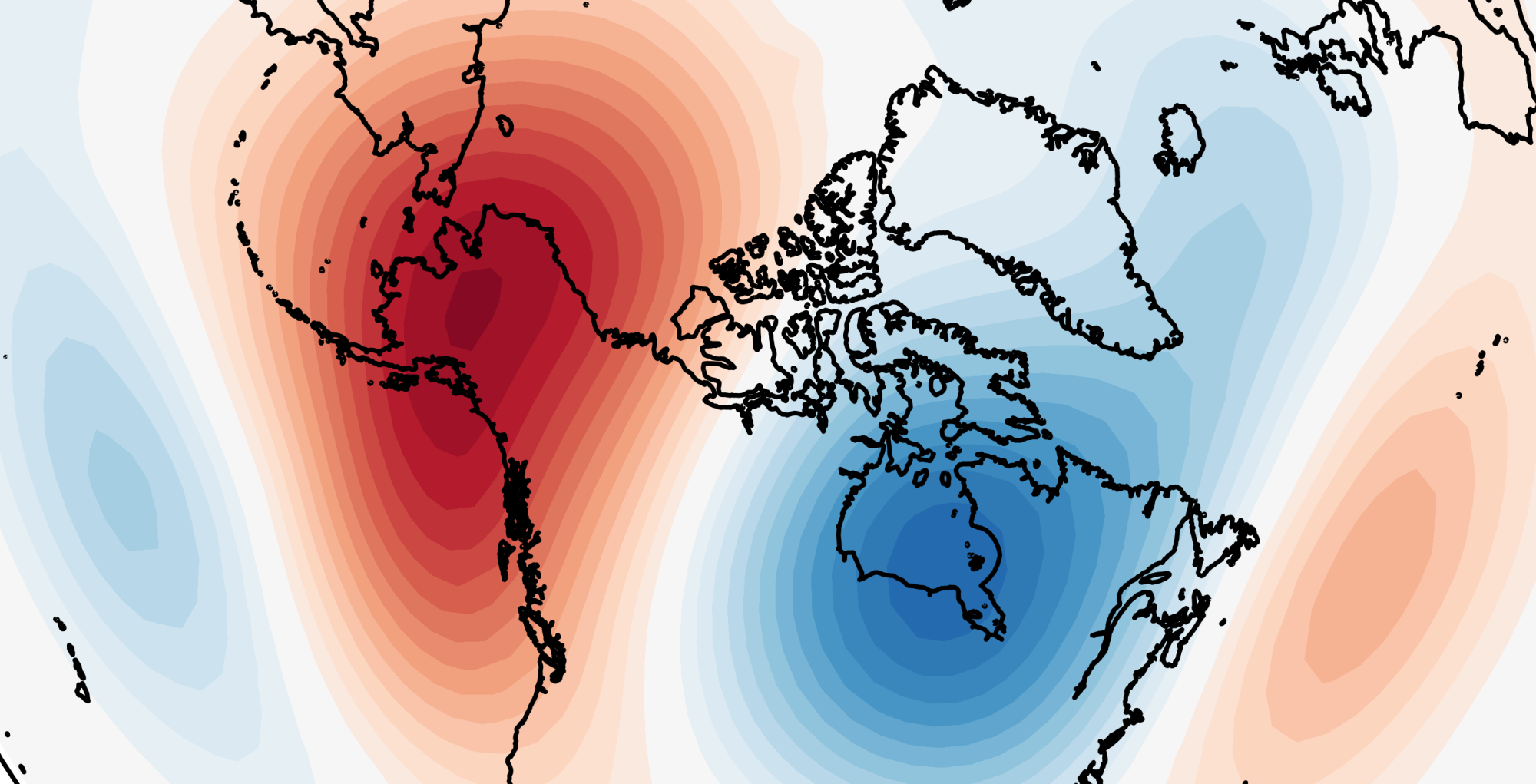
The first method is Empirical Orthogonal Function (EOF) analysis. In essence, EOF analysis decomposes a dataset into a set of uncorrelated, orthogonal patterns (as you might expect). It is performed on the anomalies of the dataset, not the full field. On any day, the field — such as MSLP or 500 hPa geopotential height — can be reconstructed by summing together a scalar loading of each EOF. The first EOF is defined such that it describes the most variability contained in the dataset, and then each subsequent EOF describes less and less (while each being orthogonal to each other). In the North Atlantic region, the first EOF of MSLP or Z500 (the “leading mode of variability”) is a meridional dipole between Iceland/Greenland and the Azores (Fig. 1) — and is thus considered the NAO.

This is primarily why the NAO gets the attention it does — because it is the leading mode. By no means is it the full picture, as it only explains around a third of the variability (or even less on daily timescales). But of all the components which make up the field, the NAO is dominant, and it’s thus a good starting point or focus for forecasts.

The EOF-based NAO has an associated index time series, produced by projecting the EOF onto the anomaly field each day, which describes the strength of the pattern. This is often normalised by some measure, such that it can be easily interpreted as standard deviations from the mean. Long-range model forecasts account for mean-state biases by calculating the EOF-based NAO on anomalies with respect to the model climate, over the hindcast period.

But the leading mode of variability is affected by the seasonal cycle — the way the MSLP anomaly field over the Atlantic varies in July is vastly different to January thanks to the seasonally-dependent latitudinal shifts of the jet. Thus, this has to be accounted for — so oftentimes an NAO pattern will be seasonally varying. It’s important therefore to remember that the EOF-based NAO+ pattern at one time of the year differs slightly to that at others (Fig. 2). For example, in the UK in January, NAO+ is likely to be stormy and westerly, while NAO+ in July is more anticyclonic with an extended ridge from the Azores.

The second method is k-means clustering to produce regimes. While an EOF-based NAO is a continuous index, clustering discretises the data. Typically, in the Atlantic during winter, four clusters are used, shown in Fig. 3; each day is then assigned to the cluster to which it is closest. Two of these four look like the NAO, so are often called the NAO+ and NAO- regime — but they are not exactly the same as the positive and negative phases of the NAO pattern (there is a North American regime which resembles NAO- that is often called “Arctic High”). The other two regimes are the Atlantic Ridge and Scandinavian Blocking. Sometimes a “no regime” classification is included, to account for days where the anomaly field does not closely line up with any of the regimes, or is very similar to more than one.

Each of the four regimes also projects onto the EOF-based NAO index, so it is possible to not be in the NAO- regime while the NAO index is negative (an extended Atlantic Ridge or Scandinavian Block can do this).

It just so happens that the second leading mode of variability (EOF) in the Atlantic is very close to the Scandinavian Blocking regime. (If you shrink the domain over which the EOF is computed to just the far North Atlantic, the result is what we call the “Scandinavia-Greenland pattern” in a recent paper.) The upshot of these two EOFs is that you can learn a bit more about the exact characteristic of the regime by plotting EOF1-EOF2 phase space (Fig. 4), where the x-axis is the NAO index and the y-axis is the Scandinavian Blocking (BLO) index (the negative of which is a Scandinavian trough). The four quadrants, clockwise from top left, are thus: NAO- BLO+, NAO+ BLO+, NAO+ BLO-, NAO- BLO-.

We can visualise this as an anticlockwise progression around the phase diagram (Fig. 5), similar to how the MJO is often considered — although the NAO/BLO cycle is rarely this continuous or smooth. Nevertheless, I think this is a pretty neat diagnostic which tells you quite a bit more than just using one in isolation, particularly in northwest Europe where the second EOF has its largest footprint.

Regimes, like EOFs, also require seasonal adjustment; seven regimes have been adopted or year-round use, while the specific decisions made in the clustering technique can also alter the outcome. One exciting recent paper led by Daniela Domeisen linked the regimes around the onset of major SSWs to the following surface weather response! And with ECMWF’s open data policy, we’re all now able to see the extended-range regimes forecasts (Fig. 6) which should provide a more insight into the subseasonal range by condensing 47 days of 51 ensemble members into simple probabilities.

So, are any of these regimes or patterns (or whatever you might call them) “real”? Well, not necessarily in terms of what we humans manage to create by our analysis techniques. No matter the science, some subjective decisions are made which slightly alter each outcome. But the atmosphere has stationary waves, and favoured modes which are excited or suppressed — these do really exist, and these pattern analyses are just our best estimates to condense the 4D atmosphere into a single number.

If you’d like to make your own EOFs in Python, I highly recommend the package eofs – https://ajdawson.github.io/eofs/latest/index.html, while scikit-learn is great for k-means clustering – https://scikit-learn.org/stable/modules/generated/sklearn.cluster.KMeans.html